GUI Walkthrough

The NEREIDS desktop application provides interactive neutron resonance imaging analysis with visual feedback at every step.

The screenshots on this page cover the current guided workflow screens: landing, load, configure, analyze, results, studio, forward model, detectability, and periodic table. When workflow labels, solver controls, or project-file behavior changes, refresh these images together with this page.

Launch

# Homebrew (macOS)
brew install --cask ornlneutronimaging/nereids/nereids

# Or pip
pip install nereids-gui
nereids-gui

# Or from source
cargo run --release -p nereids-gui

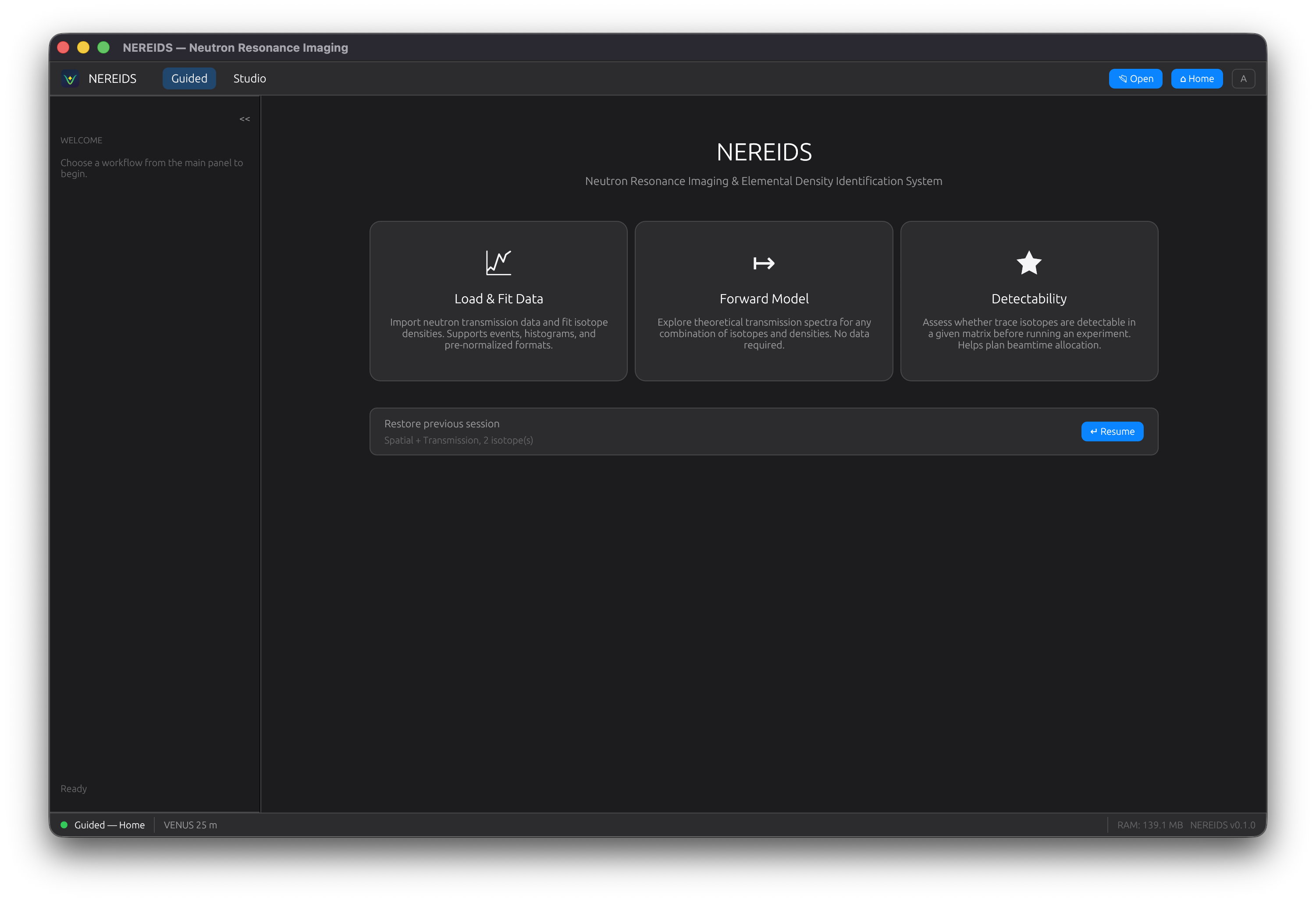
Landing Page

The landing page presents three entry points:

• Load & Fit Data – open the wizard for single-spectrum or spatial-map fitting
• Forward Model – explore theoretical transmission spectra without loading data
• Detectability – estimate trace-isotope sensitivity before an experiment

Decision Wizard

After selecting Load & Fit Data, a short wizard asks:

1. Fitting type: Single spectrum or spatial map
2. Data format: “Raw Events (HDF5/NeXus)”, “Histogram, Pre-Normalization”, or “Transmission (Already Normalized)” — quoted as the wizard cards label them

The wizard configures a dynamic pipeline with only the steps relevant to your data format. Six distinct pipelines are available.

Pipeline Steps

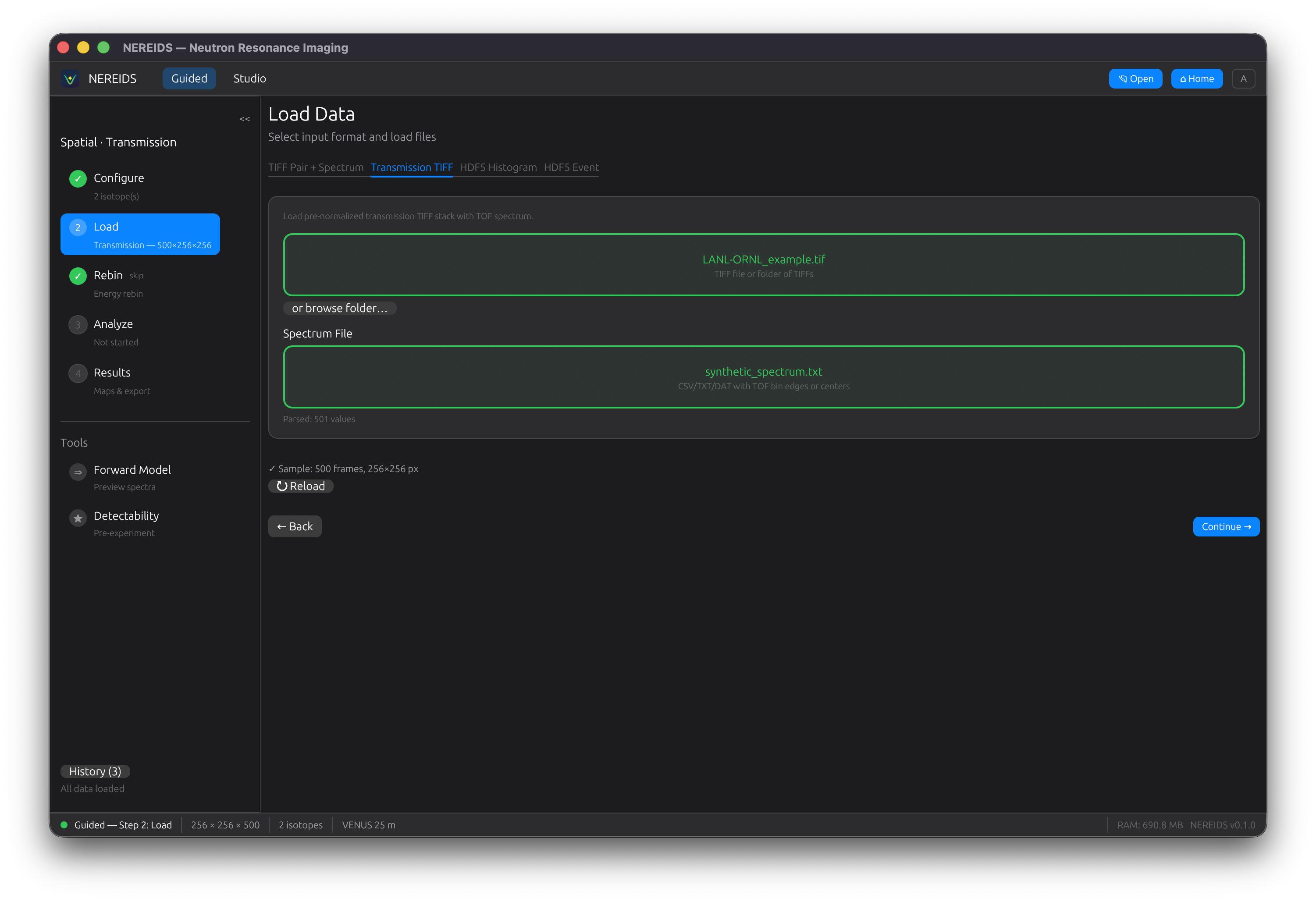
Load

Select sample data, open beam, and spectrum files. Supports multi-frame TIFF stacks, TIFF folders, and NeXus/HDF5 event data. The GUI auto-detects the file format and loads data when all fields are filled.

Normalize

For histogram/pre-normalization pipelines, including TIFF pair and HDF5 sample/open-beam counts, the Normalize step computes transmission from sample and open-beam measurements. Raw event pipelines bin events first. Transmission pipelines skip normalization because T(E) = I/I0 is already supplied.

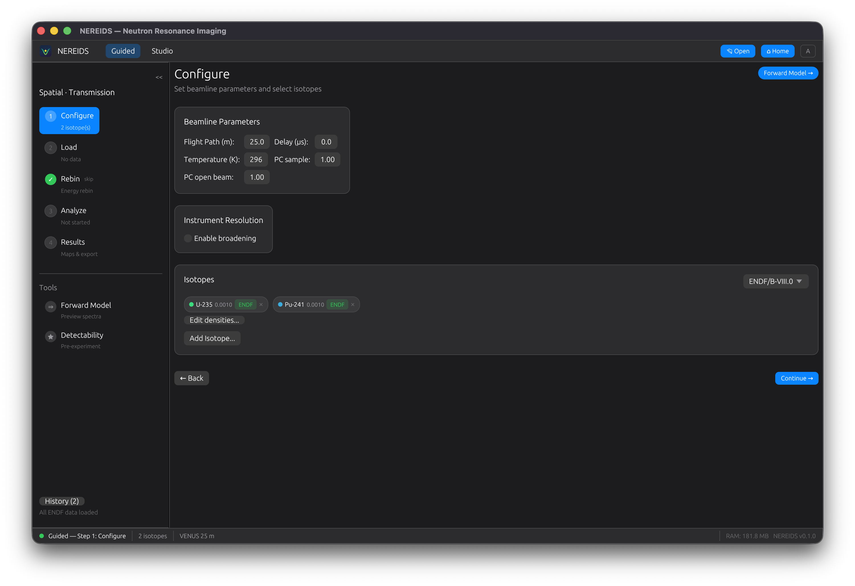
Configure

Select isotopes of interest from the periodic table. ENDF nuclear data is fetched automatically from IAEA servers and cached locally. Each isotope shows a status badge (Pending, Fetching, Loaded, Failed).

Configure beamline parameters (flight path, timing resolution) and solver settings (Levenberg-Marquardt or Poisson KL divergence).

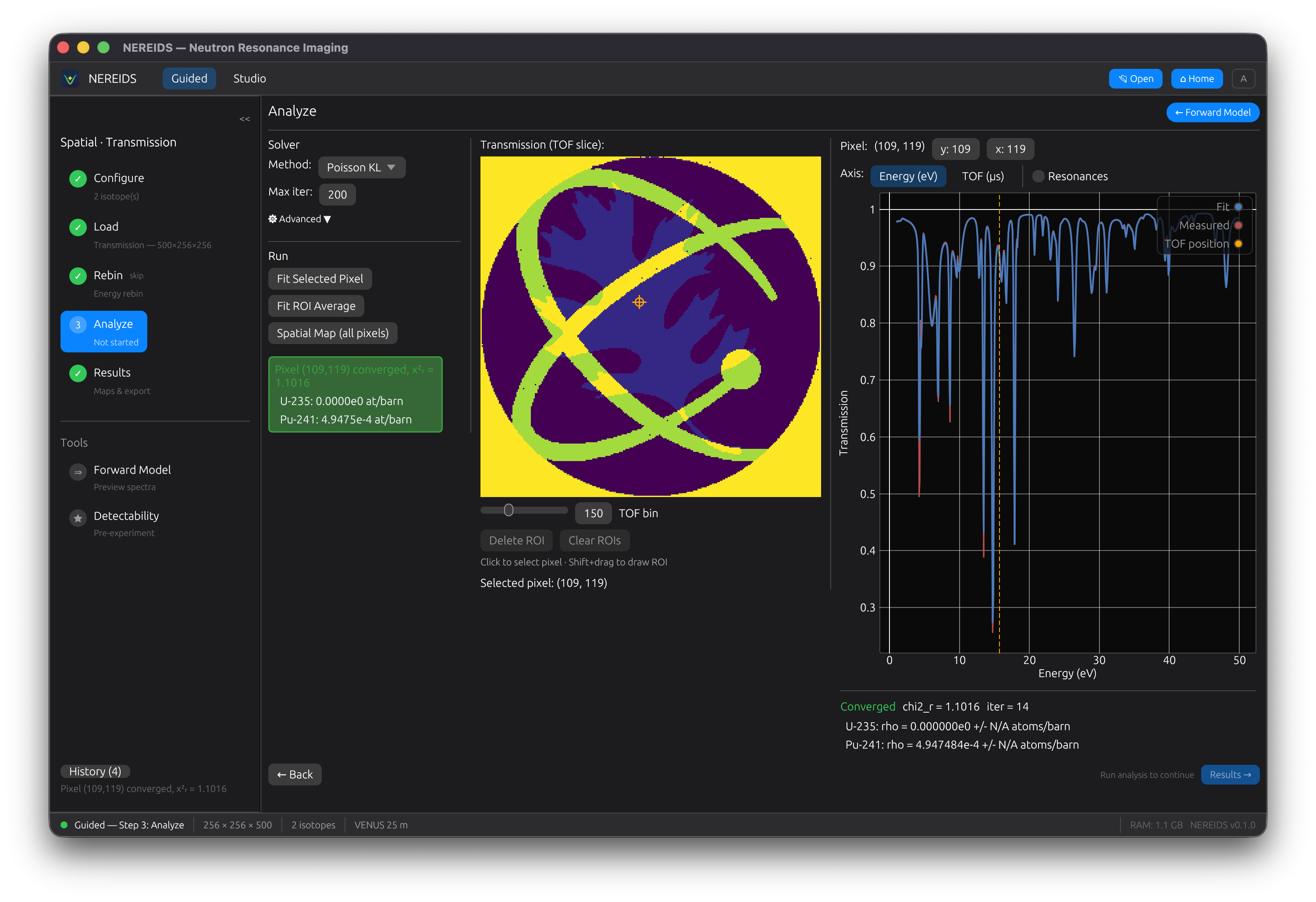
Analyze

Run the fit. For spatial maps, a progress bar tracks per-pixel fitting with rayon parallelism. Click any pixel to inspect its individual fit. Fit feedback shows green (good fit) or red (failed) status.

Draw regions of interest (ROI) with Shift+drag. Multiple ROIs are supported with move, select, and delete operations.

Restricting the fit energy range (SAMMY EMIN/EMAX)

By default NEREIDS fits the entire loaded energy grid. The advanced solver panel exposes a “Restrict fit energy range” checkbox (equivalent to SAMMY’s EMIN/EMAX analysis limits) that limits the cost function to a user-specified [E_min, E_max] window in eV. Common uses:

• Resolved-resonance region only — exclude the unresolved-resonance and high-energy tails where the model can’t fit;
• Single resonance triplet — focus on a specific feature for fine-grained density / temperature work;
• SAMMY parity — match the EMIN/EMAX restriction used in a reference SAMMY fit so the comparison is apples-to-apples.

When the checkbox is on, two grey dashed vertical lines on the spectrum plot mark the active boundaries (visible on the energy-eV axis). The reduced χ² and degrees-of-freedom reported in the fit details count only bins inside the active range.

Resolution-kernel margin (automatic): the broadening kernel pulls model contributions from outside the user range. NEREIDS handles this transparently by extending the data slice by ~5×FWHM on each side and masking the cost function back to [E_min, E_max] — so resonances near the boundaries are correctly broadened without the user picking a custom margin. This follows the same endpoint-extension principle as SAMMY’s auxiliary grid (general construction: user manual Sec. III.A.2(c); the quantitative [Emin − Wmin, Emax + Wmax] statement, with W the resolution width at each limit, appears in the Leal-Hwang procedure of Sec. III.B.2); NEREIDS uses a deliberately conservative ~5×FWHM margin.

The setting persists in .nrd.h5 project files (Option<(f64, f64)>, default None = full grid for backwards compatibility).

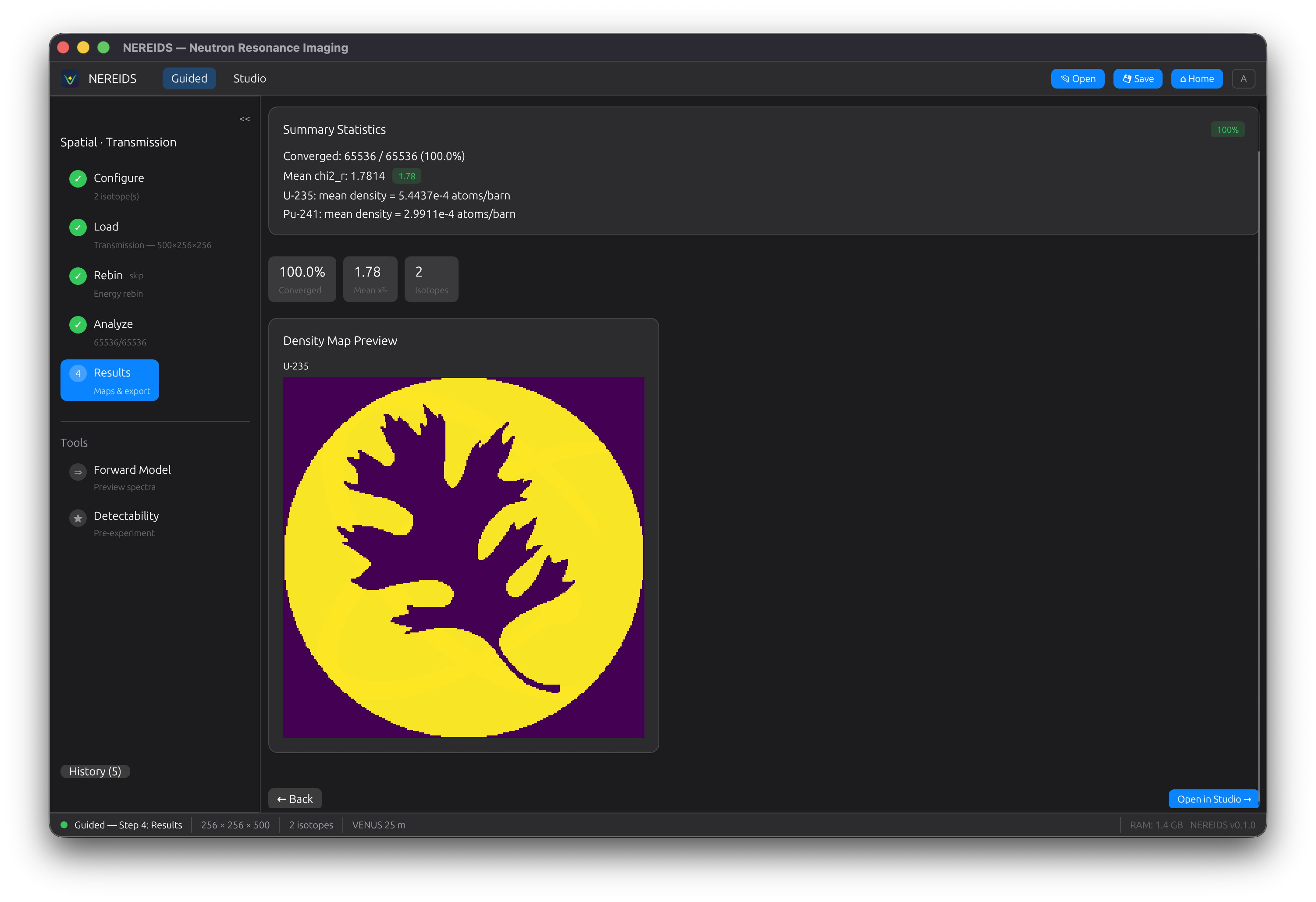
Results

View density maps for each fitted isotope. Summary statistics show convergence rate, median chi-squared, and isotope count. Open results in Studio for detailed exploration.

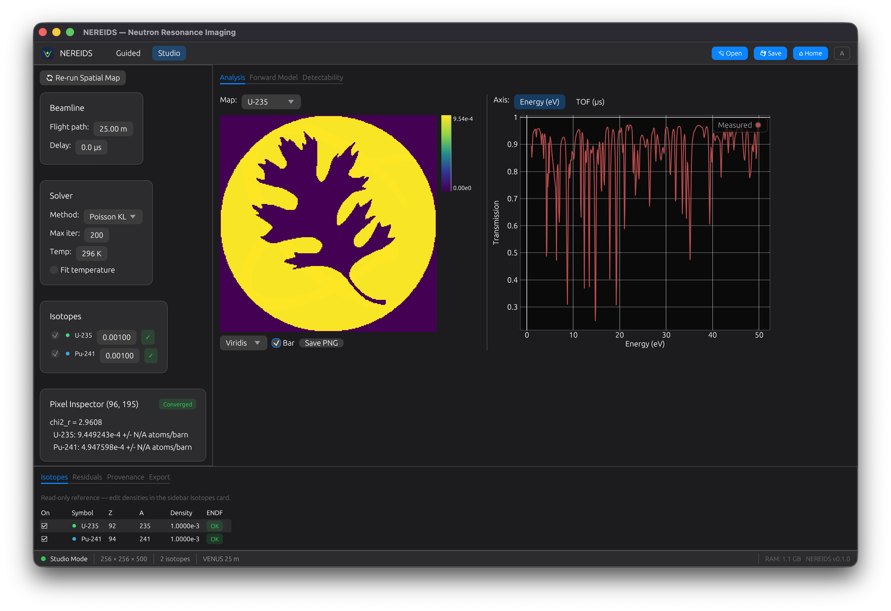
Studio Mode

Studio provides a “Final Cut”-style workspace for exploring results:

• Document tabs: switch between Analysis, Forward Model, and Detectability
• Main viewer: density map with colormap selection and colorbar
• Spectrum panel: click any pixel to see its fitted spectrum
• Bottom dock: Isotopes, Residuals, Provenance, and Export panels
• Inspector sidebar: per-pixel parameter values

Tools

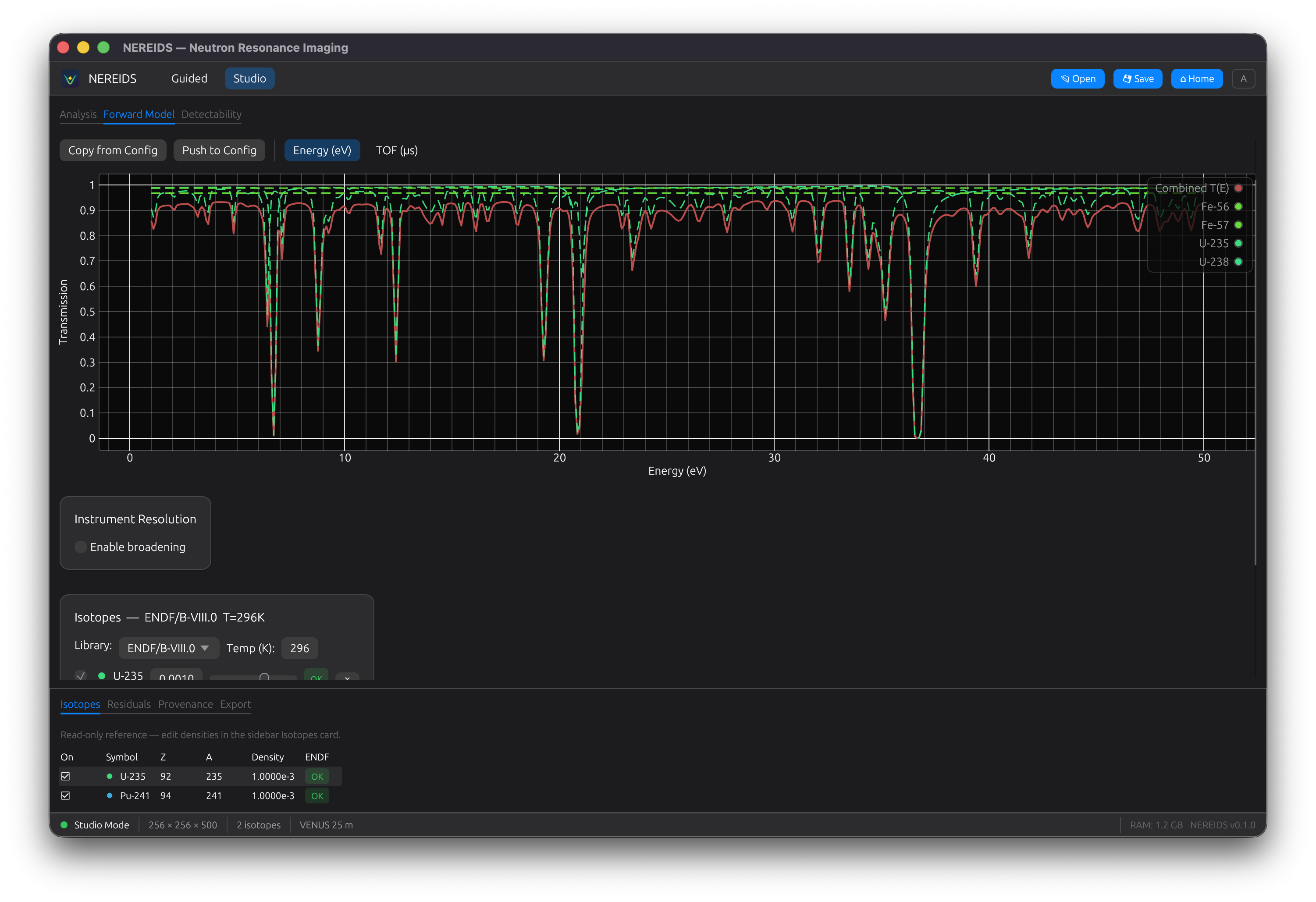
Forward Model

Compute theoretical transmission spectra for arbitrary isotope mixtures. Adjust densities with sliders and see the spectrum update in real-time. Hero spectrum layout with per-isotope contribution lines.

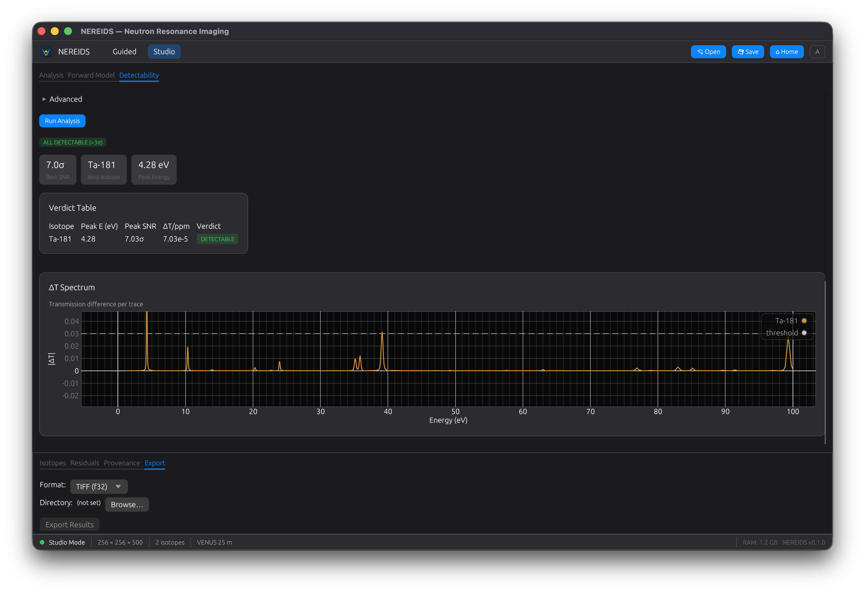
Detectability

Analyze whether a trace isotope is detectable in a given matrix material. Multi-matrix support with resolution broadening. Shows a delta-T spectrum and verdict badges (DETECTABLE / NOT DETECTABLE / OPAQUE MATRIX).

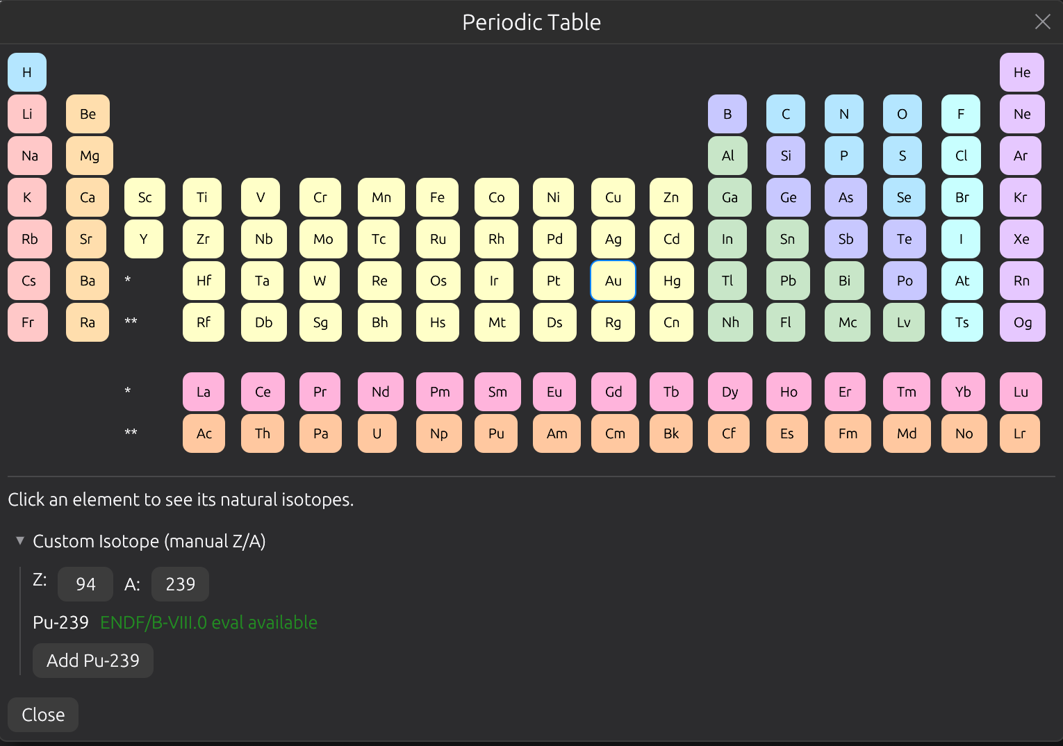
Periodic Table

Interactive 18-column periodic table for selecting isotopes. Click an element to see its natural isotopes with abundance percentages. Supports multi-select with density input. ENDF availability hints are shown for each isotope based on the currently selected data library.

Project Files

Save and load analysis sessions as HDF5 project files (.nrd.h5):

• Cmd+S (macOS) / Ctrl+S (Linux): quick-save
• File > Save: save with dialog
• File > Open: load a saved project

Project files store raw data, pipeline configuration, and results. Embedded data mode bundles everything into a single portable file.